 1 variable Newton's method
SolveNonlinear can solve nonlinear systems of equations with 1, 2, or 3 variables using Newton's method, an alternate method that approximates the (partial) derivatives, or the secant method. The (partial) derivatives are required are required for Newton's method but not for the other methods. Approximate solutions values are required for each method.
For two equations the functions have the form fi(x, y) = 0. When using Newton's method, the required information is:
  f0(x, y)
  f1(x, y)

  δf0(x, y)/δx
  δf0(x, y)/δy
  δf1(x, y)/δx
  δf1(x, y)/δy
When using Newton's method for a system with only 1 variable, a function of x and its derivative are needed. For systems of 3 equations, 3 functions of x, y, and z and 9 partial derivatives are required.
For the alternate method the (partial) derivatives are not needed but instead they are approximated using only the functions.
For the secant method, two sets of approximate solutions are required.
After entering the
required information, the user can press "Iterate" to cause one
iteration to be performed. Pressing the "Solve" button causes
iterations to continue until the sequences converge. The iterates are
printed in the canvas on the left. If the sequences converge, the final
answer is printed in red. If the sequences have not converged in 20
iterations, one of two warning messages will appear.
The iterations may be converging slowly.
You can iterate some more, if desired.
The sequences are probably converging. Clicking "Iterate" may be useful
to obtain more accuracy or confirm the solution. The message
The iterations do not seem to converge.
may indicate that better initial values are required or no solution exists.
Note: This program provides no special assistance other than terminating iterations in situations where the iterations diververge or the Jacobian at the solution is singular.
1 variable Newton's method
The extension to systems of equations is fairly obvious to those familiar
with linear algebra. For systems of two equations, let the vectors F(x, y) and
X, and Jacobian matrix be
            ⌈f0(x,y)⌉            ⌈x⌉
   F(x,y) = ⌊f1(x,y)⌋        X = ⌊y⌋

            ⌈δf0(x,y)/δx   δf0(x,y)/δy⌉
   J(x,y) = ⌊δf1(x,y)/δx   δf1(x,y)/δy⌋
Newton's method for systems of equations is
Xn+1 = Xn -
J(Xn)-1F(Xn)
The convergence is quadratic if the determinant of the Jacobian at the
solution is not 0, that is, if the Jacobian at the solution is
nonsingular. It should be noted that the calculation of
J(Xn)-1
is not needed in practice. Instead one solves the linear system
J(Xn)Yn = F(xn)
for Yn and uses
Xn+1 = Xn - Yn
The derivative of f(x) can be defined as
                    f(x + Δx) - f(x)
       f'(x) = lim  ----------------
               Δx→0       Δx
That means that if Δx is sufficiently small, then
         f(x + Δx) - f(x)
        ----------------
                Δx
is a good approximation for f '(x). The alternate method takes advantage
of this to approximate the derivative and the approximation is used in an
almost Newton's method for 1 variable problems. The concept is used to
approximate the partial derivatives needed in systems with 2 or 3 variables.
The convergence is nearly quadratic but sometime an extra iteration or
two is required. The convergence criteria is more stringent and sometimes
an extra iteration used but it often results in no change in the solution.
Comments:
Efficiency: The approximation method replaces the evaluation of
(partial) derivatives with the calculation (1 variable)
(f(x + Δx) - f(x))/Δx.
f(x) has to be calculated anyway so for each (partial) derivative
there is 1 additional
function evaluation, 1 subtraction, and 1 division instead of
evaluating the (partial) derivative itself. In general, this is not a
significant difference.
Number of iterations: In experiments done so far, the number
of iterations is rarely increased by more than one with an appropriately
sized Δ.
The approximation method: In this program, the approximations
of the (partial) derivative is done with a simple, one side approximation.
It would be possible to make better approximations. For example, one
could use (f(x+Δx) - f(x-Δx)/(2*Δx). While
this would allow a larger Δx, it requires calculating
a third function (f(x-Δx)) in addition to the two
required for the simpler approximation but it would rarely decrease the
number of iterations needed to solve the problem.
Size of Δ: The program supplies a default value of
Δ of 0.0001 which is arbitrary but often seems to work well. The
user can easily replace the default value(s), if desired. While
it is a pretty simple problem, consider the following table showing the
number of iterations needed to obtain 16 decimal places of accuracy when
using f(x) = x2 - 4 starting with
x = 3.
      Δx     Number. of iterations
      1          20
      0.1        10
      0.01        8
      0.001       6
      0.0001      6  (same as Newton's method)
      0.00001     6
(Sometimes an additional iteration is shown but with no change in the x value. Actually, it uses 6 iterations with Δ anywhere from 10-3 to 10-12)
Clearly this is a simple problem but it gives some idea of desirable values of Δx. We would not normally recommend a much smaller value because the approximation requires subtracting to nearly equal functional values. This can lead to problems of significance. Fortunately the calculations are done in double precision. The method is not recommended if single precision calculations are used.
 1 variable secant method
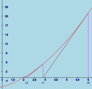
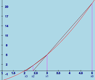
The one variable secant method is well known and is sometimes used because it does not require the derivative. Instead it uses two approximate solutions. The method can be thought of as follows. Given two approximate solutions, draw a secant line between the two functional values at those approximate solutions. The point where the secant line touches the x axis is the next approximation and the oldest approximate solution is discarded. The disadvantage is that even when the derivative is not zero at the solution, it converges at a rate that is less than quadratic even though it is much faster than linear.
The secant method was extended to 2 or more variables. Its convergence rate is similar to the 1 variable situation.
Because the convergence is less than quadratic, more iterations are normally required than for either of the other methods.
For Newton's method, if the sequence converges quadratically, the number of correct decimal doubles with each iteration. The convergence criteria in this program is designed so that the final values are normally correct to the number of decimal places shown. However, this may not be true when the convergence is linear.
For the alternate method, the convergence criteria in the program is sharpened. When the convergence is nearly quadratic, the results show are normally accurate but some times an extra iteration may be shown. Again when the convergence is linear, the final result may not be the best possible.
For the secant method, the convergence criteria is even sharper. One can check the "final" answer with another iteration if desired.
The following table compares some iterations for solving y = x2 - 4 starting with x0 = 4 and x1 = 3.5 for the secant method . Value are rounded to avoid showing lots of unneeded digits. Initial approximations are shown in green, final answers in red.
     Newton's Method      Approximation          Approximation        Secant
                          with Δ = 0.0001        with Δ = -0.0001
 0   4.000                4.000                 4.000                4.000
 1   2.500                2.50002               2.49998              3.500
 2   2.0500               2.050012              2.049987             2.400
 3   2.000610             2.000611              2.000608             2.102
 4   2.0000000929         2.000000109           2.000000077          2.0090
 5   2.0000000000000022   2.0000000000027       1.9999999999980      2.00022
 6   2.0000000000000000   2.0000000000000000    2.0000000000000000   2.000000504
 7                                                                   2.0000000000282
 8                                                                   2.0000000000000000
Discussion: One can see that the convergence of the approximation methods with this simple problem is nearly as good as with the true Newton's method. Because of the concavity of the curve, using Δ = .0001 slightly over estimates the derivative resulting in slightly larger iterate values while using Δ = -.0001 slightly under estimates the derivative so the resulting iterate values are slight smaller. But in end, the sequence converges in the same number of steps for the first three examples. For these two initial values, the secant method takes one additional iteration. (Step 1 is an initial guess.) It converged in the same number of iterations when the second approximation of 3.5 was replaced by 2.5 .
The following is a 3 variable problem presented in
www.lakeheadu.ca/sites/default/files/uploads/77/docs/RemaniFinal.pdf
by Courtney Remani.
3 * x - cos(y * z) - .5 = 0
x2 - 81 * (y + 0.1)**2 + sin(z) + 1.06
e-x * y + 20 * z + (10 * π - 3)/3
The convergence criteria was 10 decimal places.
               Newton's Method                                Approximation
                                                              with Δ = 0.0001
         x             y              z                x              y               z
 0  0.1            0.1           -0.1              0.1            0.1            -0.1
 1  0.49987        0.0194        -0.522            0.499987       0.0195         -0.522
 2  0.5000142      0.00159       -0.52356          0.5000143      0.00160        -0.5236
 3  0.500000114    0.0000124     -0.52359845       0.50000012     0.0000134      -0.5235984
 4  0.5000000000   0.0000000008  -0.5235984756     0.5000000001   0.0000000076   -0.5235987754
 5  0.5000000000   0.0000000000  -0.5235987756     0.5000000000   0.0000000000   -0.5235987756

               Secant Method
         x             y              z
 0  0.1            0.1           -0.1
 1  0.2            0.05          -0.2
 2  0.49998        0.0094        -0.5228
 3  0.500017       0.0018        -0.52355
 4  0.50000074     0.000081      -0.523597
 5  0.5000000067  -0.00000073    -0.52359876
 6  0.5000000000   0.0000000003  -0.5235987756
 7  0.5000000000   0.0000000000  -0.5235987756
Discussion: The convergence rate for the approximate method is nearly identical to Newton's Method. The series converged in 6 steps with Δ = 0.001 but took 8 iterations with Δ = 0.01 .
The secant method took 1 additional iteration with the second guess as shown. (Again step 1 is an initial guess.)
Sometimes additional iterations were carried out without any change in the values.
The example problem "Parabola with almost a double root.", f(x) = x**2 - 2 * x + 0.9999, was designed to "stress test" all three solution methods. It presents several numerical problems.
As a result, even Newton's method can only achieve 14 decimal places of accuracy compared with at least 16 when solving x**2 - 1. Newton's method solves the easier problem in 5 iterations starting with x = 1.5 compared to 10 in the harder problem.
The approximate method is a little slower in solving the harder problem taking 12 iterations with Δ = .0001= 10-4 compared to 10 with Newton's method when starting with x = 1.5. But only 10 iterations were needed when Δ is in the range of 10-6 to 10-10. That is the same as for Newton's method. This shows that it is possible to use a Δ even smaller than .0001 in some problems. (The program normally shows one extra iteration because of the strict convergence criteria for this mode.)
The secant method took 13 iterations even when the second guess was very close to Newton's method's first iteration result.
When writing functions: The operational signs are +, -, *, /, % and **. You can use ( and ) to control the order of operations and with functions.
The % operator means modulus. That is, if we have a % b we would divide a by b as integers and the result is the remainder. For example, 13 % 3 = 1 as 13 divided by 3 is 4 with a remainder of 1. Some more examples: 11 % 5 = 1. 215 % 10 = 5
The ** operator means "to the power". Thus, 3**2 = 9, 2**3 = 8, and 10**3 = 1000. 2**2**4 = 2**16 = 65536.
You can use some constants: PI (π = 3.141592653589793), QUARTER_PI, HALF_PI, TWO_PI, Math.E (e = 2.718281828459045).
Some of the functions that can be used follow. (Note: some of these functions are not differentiable and can't be used in SolveNonlinear functions.)
Order of evaluation:
Illegal values like sqrt(-2) and 1/0 are ignored.
After you finish typing a function, press "Enter".
Formulas can contain comments using // and /*...*/.
This button is useful if you have a copy of SolveNonlinear on your computer. If you set up a problem that you want to use again in another session, you can click this button and dialog box will show the information needed for the current problem to add it to the setupExamples() function in the SolveNonlinear.pjs. Some browsers (e.g. Firefox) will allow you to copy the information and paste it into the function. Because some browsers do not allow copying from the dialog box, you will be given an option of saving the information to a file. If you select this option, some browsers will give you options about what should be done with thee file. When you copy this information into setupExamples, you will have to provide an unique example number and a name for the example. Formulas are shown in the order of the example numbers.
If you click this button, the current setup is saved as a new example which is added to the list of examples. You will be required to supply a name for the new example. The temporary example will only be available for the rest of current session.
solver
Solves one dimensional f(x) = 0 by several methods.
solve linear
Solves linear system of equations with one or more right hand sides
allowing it to find
inverse matrices. Note: SolveNonlinear can also solve linear systems of
equations in one step. The Jacobian is just the coefficient matrix.
This program uses the same linear algebra library routines as solve linear.
©James Brink, 11/19/2021