 The secant method
Solver solves f(x) = 0 using either secant method, Newton's method or several variants of Newton's method some of which can automatically detect multiple roots and speed iterations. The variants include
Methods 3 and 4 are "well" known (en.wikipedia.org/wiki/Newton%27s_method).
While the methods to solve functions with multiple roots are mathematically great, there is often disappointment that mathematical calculations at roots with multiplicity result finding those roots with less accuracy than hoped even though the calculations are done with double precision.
It graphs the function and the iterative steps. There are some tests that may help when the iterations do not converge. Optionally, it can graph the first and second derivatives of the function.
Another option is provided for solving cubic (as well as quadratic and linear) polynomials analytically (without iteration). It uses a complicated set of formulas to find all the exact real solutions without requiring any starting values.
Graphing the function may be helpful in select starting points for the iteration and showing the iterations graphically may be helpful in understanding the method.
To use the solver, one supplies the function and its first and second derivative as needed. The secant method and the methods that use approximate derivatives do not require a derivative. The first derivative is required for the Newton's and the accelerated method. Both the first and second derivatives are required for the modified method and the iteration with g(x) = f(x)/f'(x) requiring g'. The user also supplies an initial guess or guesses at the root.
This apt is based on the grapher apt but only the rectangular mode is supported. While the functions are labeled differently, one can actually graph up to the 6 functions that grapher allows if it is not desired to solve f(x) = 0.
It is best to make sure that "Allow motion" is not checked before typing anything to change any of the input boxes.
The white area above the plot is used to display the results of iterations for iterative methods and the solutions when the cubic method is used and some messages. The line for iterations and solutions contains:
See Options for special features. below.
The first 3 function input boxes are labeled f(x), f '(x) and f ''(x). The fourth box has several different uses. It holds the code for the drawing tangent lines drawn when using Newton's and related methods. When using the secant method, it has code for the secant lines. In the accelerated method is used, the label changes to "iter line" because the line is no longer tangent when an accelerator is used. The fifth function box labeled "v line" holds the code for the vertical lines for the iteration methods. The normally unlabeled last function box, is label "quad" box, when it holds the code for the pieces of quadratics (parabolas) for the modified Newton's iteration steps. It changes to g(x) when one of "use g(x)" methods are used.
Use x for the independent variable.
Note: If the "f(x)" function box is changed and you press "enter", then the "tangent" and "v line" boxes are cleared in order to clear the graph of any previous solution's iterations because those iterations no longer apply. In addition, the last function box is cleared if the last solution method used that box.
It is possible to use the 6 function input boxes to plot 6 different functions if you do not want to use the "Solve" methods. Just remember to check the Show f ' and Show f '' boxes to show the functions in the second and third function boxes. (But change the first function box before the third, fourth, and fifth boxes because changing the first box clears the third and fourth (and sometimes the last) boxes as noted above.)
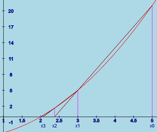
The secant methodThe secant method uses interpolation of two data points on the curve to find the next iterate. Geometrically, the method can be explained as follows. If xi-1 and xi are iterates, then xi+1 is determined by drawing a line through the points (xi-1, f(i-1)) and (xi, f(xi)). xi+1 is the intersection of that line and the x-axis. The convergence is typically fairly fast for simple roots but slow for multiple roots (i.e. when f '(x) is also zero). In fact, the convergence rate can be shown to be the Golden ratio ≈ 1.618 if the derivative is not zero at the solution.
 Newton's method
The geometric concept of this method is to draw a tangent line to the
function at a xi value. The next iterate value xi+1
is at the location where the tangent line crosses the x axis.
Mathematically, the formula is
xi+1 = xi
- f(xi)/f '(xi).
If the derivative at the
solution is not 0, the method converges quadratically and the
number of correct decimal places in the approximate solution about
doubles with every iteration.
The method can be derived by expanding the function
in a Taylor series about the solution. If x is a solution of f(x) = 0
and xi is an iterate, then
0 = f(x) = f(xi) + f '(xi)(x - xi)
+ f ''(xi)(x - xi)2/2 + ...
If you ignore the second and additional derivatives, solve for x, and
then set x to
xi+1, you get Newton's iteration formula.
Normally, the iteration converge quickly if the initial guess is close. However, if f '(x) also is 0 (a multiple root), the iterations will converge slowly.
Show proof that Newton's method converges quadratically.This method approximates f '(x) with (f(x + delta) - f(x))/delta where delta is 10-6. The convergence rate closely approximates Newton's method and typically converges in the same number of steps as the true Newton's method. The value of delta is arbitrary but normally works very well. A two sided approximation of f ' would could be used but does not seem necessary and would require an extra evaluation of f(x - delta).
Using the single sided approximation method is about as efficient as the regular method because the calculation of f '(x) is replaced by the calculation of f(x + delta) with an extra subtraction and division. (Calculating f(x) is required by either method.)
This app uses double precision. It would not be recommended for single precision especially not with the value of delta as small as the one used in this app.
Warning: This method is not recommended for finding a multiple root.
Snow a mathematical analysis of the approximation method.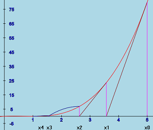 Modified Newton's method used on
 0 = f(x)
= f(xi) + [-f''(xi)(x - xi) + ...](x - xi)
+ f''(xi)(x - xi)2/2 + ...
= f(xi) - f''(xi)(x - xi)2/2 + ...
which meansThere remains a question: How do we know when to use the modified
method? If one looks at the iterations, the situation is pretty
obvious. But how can the computer make the decision automatically? It
is known that when f '(x) = 0, the regular Newton's method converges
linearly in this situation. Thus
xi/xi-1 ≈
xi+1/xi.
Hence, while iterating with
the regular Newton's method, if the computer observes that
|xi/xi-1 - xi+1/xi|
is small, then it is wise to switch to the modified method.
Unfortunately, the modified iteration does not have the nice geometrical interpretation as the regular iteration. If we look at the above formula for (x - xi)2 and ignore the "+ ..." we have a quadratic function that has zeros at the x values given by the ± in the above formula for xi+1. The plot of the modified method shows the half of this parabola between the last xi value and xi+1.
In practice, the f(xi) / f''(xi) is almost always positive in the case of double roots, allowing its square root to be calculated if xi is close enough to the solution.
Warning: When trying to solutions to functions at a multiple
root, accuracy of the result is limited by numerical problems. For
example, when the solving
f(x) = x(x-1)2 = x3 - 2x2 + x = 0
as shown in the picture at the beginning of this section. Clearly,
x = 1 is a double root. But
starting at x = 5, the iteration stopped at
x8 = 0.99999999883
because it calculated f(0.99999999883) = 0 even though double
precision arithmetic was being used.
 Accelerated Newton's method
  n     xn           Δn        Δn/Δn-1
  0    2.0000
  1    1.6000      0.4000
  2    1.3474      0.2526      0.6315
  3    1.1935      0.1539      0.6093
Clearly the number of correct decimal places is not doubling with each
iteration. In fact, each difference is very roughly 6/10 of the previous
difference. (If we continued this process, the ratio converges to
1/2.) This means that iteration is not converging quadratically and is, in
fact, showing
roughly linear convergence. This suggests that we have a double root and
the convergence is only about half what would be expected for quadratic
convergence. So might decide to accelerate the convergence by multiplying
the normal Newton's method difference by 2 and calculating x3
using
x3 = x2 - 2 * Δn
= 1.3474 - 2*(0.1539) = 1.0396
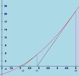
We will call this process accelerated Newton's method. This acceleration
is shown in the picture. The normal tangent is used at x0 and
x1. However, at x2, Δ2 is doubled and
x3 is much closer to the root at x = 1 than the original
x3 calculated by Newton's method.
The concept can be expanded to higher order roots. For example,
for triple roots, Newton's method converges linearly with
Δn/Δn-1 is roughly 2/3. With
quartic roots, Newton's method converges linearly with
Δn/Δn-1 is roughly 3/4. The program
tries to guess triple and quartic roots and is sometimes successful. When it
does, it multiplies Δk by an acceleration factor of 3 or 4.
But there are some
limitations. If it guess wrong, the sequence may not converge. Even if the
sequence converges, numerical issues often mean that results are not
as accurate as might be desired.
The method solves simple problems such as (x - a)k = 0
for k = 2, 3, and 4 in one accelerated iteration just as the regular Newton's
method solves (x - a) = 0 in one iteration.
Warning: When trying to solutions to functions at a multiple
root, accuracy of the result is limited by numerical problems. For
example, when the solving
f(x) = x(x-1)2 = x3 - 2x2 + x = 0
as shown in the picture at the beginning of this section. Clearly,
x = 1 is a double root. But
starting at x = 2, the iteration stopped at
x6 = 0.9999999995
because it calculated f(0.9999999995) = 0 even though double
precision arithmetic was being used. The situation can be even worse when
there is an even higher order root.
.png) Iterating with g(x). Note: the red curve is the original f function. The dark
blue curve is g(x) which was processed by Newton's method.
Iterating with g(x). Note: the red curve is the original f function. The dark
blue curve is g(x) which was processed by Newton's method.
Unfortunately, applying Newton's method to g(x) requires a second derivative of f(x). Because, if g(x) = f(x)/f'(x), then
g'(x) = [f'(x)f'(x) - f(x)f''(x)]/f'(x)2
                  = 1 - f(x)f''(x)/f'(x)2
This apt will automatically calculate g and g' when f, f ' and f '' are
provided so that Newton's method with g(x) can be carried out. The g(x)
function is added to the last function box allowing the iterations with
g(x) to be shown in the graph.Because g '(x) is quite complicated, using approximate derivatives seems quite attractive. It normally converges in the same number of steps. The comments in the previous section are still appropriate.
(This method can also find solutions of quadric and linear equations.)
Methods for solving cubic polynomials have been studied for centuries. Unfortunately, the methods are rather complicated and seldom used. This program uses a method that transforms the general cubic into a special form t3 + pt + q = 0 which has a known (but complicated) solution. The solutions for the transformed equations then can be used to obtain solutions of the original cubic equation with analytically without iteration. The method uses code published by Alexander Shtuchkin.
Assume the cubic equation is written in the form ax3 + bx2 + cx + d = 0. To use this method, the values of a, b, c, and d must be provided in the values boxes below the graphing area and the "Solve (Cubic Method)" is clicked. The cubic and its first 2 derivatives are displayed in the function boxes and function (and optionally the derivatives) are shown in the graphing area. The solutions are displayed in the result area. There is no need to type in functions or starting values. (Quadratic and linear equations can be solved by just setting a and b = 0, as needed.)
Because clicking "Solve (Cubic Method)" writes the function and its derivatives in the first 3 function boxes, the problem can then be solved by any of the other solution methods, if desired.
Note: If the cubic example is selected, then the cubic solving method is automatically selected. (This is invoked by setting the mode in the example to 1.)
Occasionally, a "Continue iterating" button will appear below the solve buttons. This happens if the iterations are terminated for some reason, but the final value of the function does not seem small enough. Often the reason is numerical accuracy and the additional iterations do not help. But in some cases they may help.
When writing functions: The operational signs are +, -, *, /, % and **. You can use ( and ) to control the order of operations and with functions.
The % operator means modulus. That is, if we have a % b we would divide a by b as integers and the result is the remainder. For example, 13 % 3 = 1 as 13 divided by 3 is 4 with a remainder of 1. Some more examples: 11 % 5 = 1. 215 % 10 = 5
The ** operator means "to the power". Thus, 3**2 = 9, 2**3 = 8, and 10**3 = 1000.
You can use some constants: PI (π = 3.141592653589793), QUARTER_PI, HALF_PI, TWO_PI, Math.E (e = 2.718281828459045).
You can use some values: a, b, c, d, e, and s. They will be explained in the values section.
Some of the functions that can be used follow. (Note: some of these functions are not differentiable and can't be used with Newton's method.)
Order of evaluation:
Illegal values like sqrt(-2) and 1/0 are ignored.
After you finish typing a function, press "Enter".
Formulas can contain comments using // and /*...*/.
There 7 options that can enhance a graph - vertical lines, rays through the origin, circles, line segments, quadratics, points, and words (labels or text) but they cannot be used in writing the function or its derivatives. The line segment option ("L") is used to illustrate secant and Newton's method iterations. The quadratic option ("q") is used in the modified method.
Values are separated by ";".
Words are centered horizontally at the specified point and are located just above the specified point.
(This option would be better named "label" or "text". But using the first letter of these names would not work because "l" and "t" have other meanings.)
It is possible to include variable values in words. The variable values are denoted by ^a, ^b, ^c, ^d, and ^e. E.g. if d currently = 3, then the "word" "value=^d stars" results in "value=3 stars".
When supplying a label for a curve, it may be desirable to have
the label's color match the curve's color. This is possible. One
needs to follow the last "word" in the input box with
; color; color number;. E.g.
w 2; 3; aWord; color; 1;
This says to put "aWord" at (2, 3) with the same coloring as function
f1. Notice the ";"s in the statement. The final ";" is absolutely
needed. It is possible to use formulas for the curve number.
Common notes:
The "x=", "o=", "r=", "l", "q","p", and "w" must be the first character(s) in the field. After that spaces are optional. In these special cases, "x", "o", "r', "l", "q", "p" and "w" can be capitalized.
The different elements are separated by ";". Failure to use ";" may cause strange errors or the item may be ignored.
You can use formulas for the numerical values. They are evaluated the same way regular formulas are evaluated - just avoid using "x", "o", or "t" in the formulas (and ";" in words).
Minimum x and Maximum x
are the left and right end points of the x axis. If the input boxes
are blank, the default values are -5 and 5.
Minimum y and Maximum y,
if specified, are the end points of the y axis. If these fields are blank,
appropriate values will be calculated automatically based on the y values
of the function.
If "Equal spacing" is true (checked) then the mins and maxs for x and y will be adjusted as needed in order to make the equal spacing possible.
Note: After you finish typing a minimum or maximum, press "Enter". The minimum and maximum values can be formulas which are evaluated the same way functions and values are evaluated. Just don't use x, t, or o in the formulas.
Sometimes it is useful to zoom in to see the iterations more closely. The Zoom In button does this. The domain is reduced by one fifth and centered at the last iteration (typically a solution). If both the y minimum and y maximum are specified the range is reduced in a similar manner. Otherwise the range is determined in the usual manner. Unfortunately, the iterations that are sometimes outside the new domain and range and not shown but may prevent the range from zooming in appropriately. The are two possible solutions. 1. Restart the iteration within the new range. 2. Specify the y minimum and/or y maximum to show the appropriate range.
If the problem has not already been solved, the zoom will center on what ever value x happens to have. The user can set the center by double click at the desired point.
Zoom out increases the domain by a factor of 5.
When Equal Spacing is checked, the units on the x and y axis are the same so a 45o line would look like a 45o line and circles will look like circles.
For the sake of efficiency, Solver stops redrawing graphs when nothing is changed. Checking Allow motion says to keep drawing. This is useful, for example, if one uses frameCount. E.g. 5 * sin(x + frameCount/10) or if you use the "s" slider. This is rarely useful when using solver.
The standard canvas is medium sized to allow the user see the canvas and many of the controls at the same time without having to scroll. This is convenient while solving problems. But a larger graph is drawn above the original canvas and controls when the "Show enlarged canvas" item is checked or the "Enlargement ratio" is changed. When using this option, one will normally have to scroll up to see the larger graph and scroll down to see the original canvas and the control items. The enlarged canvas shows a magnified image of the original canvas except text elements are the same size as in the original.
Notes:
The Radians and Degrees radio buttons allow the user to specify if the trig functions and trig inverse functions assume radians or degrees. The default is radians. Radians are required when using Newton's or the modified Newton's methods.
You can supply values for a, b, c, d, and e which can be used in the functions and other input boxes. The default value of these values is 0 when the input box is blank. They are evaluated the same way functions are evaluated. Just don't use x, t, or o in the formulas. See below for the special s value. You can use the value of one of the variables in another. For example, the expressions for a and b might be s/10 and 2 * a. Because one can use formulas for variables a, ...,e, the numerical values for these variables (rounded to 3 decimal places) is shown below the values.
The slider moves from 0 to 100 and is always an integer. If you move the slider, its value is sent to the s value input box. One can type a value from 0 to 100 in the s value input box to adjust the slider to that value. Anything else typed into that s value box is ignored and will be replaced by the value of the slider.
If the value range of the slider is not appropriate you can do something like the following: f1(x) = b * sin(x) where b value is set to s/10.
Important note: When "Allow motion" is false (not checked) the value of s is set when the mouse releases the slider but the value of s does not track the slider while the slider is moving. However, if "Allow motion" is true (checked) (and at least one function has been defined) the value of s tracks the slider.
The initial value of 200 is almost always adequate as that means the functions are evaluated at about every other pixel in the x direction.
This button may be valuable if you have a copy of Solver.pjs on your computer. If you set up a graph that you want to use again in another session, you can click this button and dialog box will show the information needed for the current plot to add it to the setupExamples function in the solver.pjs. Some browsers (e.g. Firefox) allow you to copy the information and paste it into the function. You will have to provide an unique example number and a name for the graph. Formulas are shown in the order of the example numbers. Because some browsers do not allow copying contents of the dialog box, you will be offered a chance to save the setup information to a file. If you elect this option, your browser may offer options about what to do with the file.
If a "," is included in a "word" special option w in function boxes, it will be replaced by "^$". The substitution is required because ","s are used to separate items in the data. However, this is not a problem because the "^$" is automatically replaced by "," when used in a example.
Note: If you use this technique to save a solve using the "cubic" method, you may want to change the "0," line to "1," so that the apt will recognize that it is a cubic problem and to treat it accordingly. Otherwise, it will be treated as a regular problem which can be processed by any of the solve methods.
If you click this button, the current setup saved as a new example which added to the list of examples. You will be required to supply a name for the new example. The temporary example will only be available for the rest of current session.
After finishing a graph, it can be saved as an image file. Click the button. If the enlarged canvas is being shown, the enlarged canvas is saved. Depending on your browser, you may be asked if you want to save the file. In any case, you will probably find it your normal download folder with name solver.jpg. If you save more than one time, the multiple copies will normally be numbered. Your browser may have a button to give direct access to this folder.
When the user types invalid info into one of the input boxes, a message is displayed on the top of the plot area. After fixing error, normally the error message will be hidden. Occasionally it may be necessary to click anywhere in the plot area to hide the message.
James Brink, 11/30/2021.