
DiffiEq2 can graph numerical solutions for two types of differential equations using four different numerical solution methods:
It can also plot analytical solutions to those problems when the solution(s) are known so one can compare the accuracy of the numerical solution to the exact solution.
The four numerical differential equation solvers are:
This apt is based on the Grapher apt but only the rectangular mode is supported. While the functions are labeled differently, one can actually graph up to the 3 functions in addition to the numerical solution of the differential equation or system.
It is best to make sure that "Allow motion" is not checked before typing anything to change any of the input boxes.
While the derivation of numerical methods for numerically solving differential equations can get quite complicated, the general idea is that a polynomial is used to approximate the solution and the next iterate is based on the value of the polynomial at that x value. For methods of order one, the polynomial is just a linear polynomial of order 1 (i.e. a straight line). For second order methods, the polynomial is a quadratic polynomial of order 2. Likewise, a 4th order polynomial is used for order 4 methods. Consequently, if the exact solution of the differential equation is a 2nd order polynomial like y= x2, a second order method will give an exact solution. Likewise, if the solution y is a 4th order polynomial like y' = x4, 4th order methods will yield an exact solution. Examples 4 and 5 illustrate this. In the fourth example, initially c is 0 and the solution is a 4th order polynomial and the numerical values are exact. However, if c is changed to a non-zero value, the solution is 5th order and the numerical solution is very close but no longer exact. You will have to use one of "Show data" options to verify these claims.
Interestingly, even though the theory would suggest that error depends on the solution, not just the y' formula, in practice those examples show the if the y' formula includes y as well as the independent variable x, very small numerical errors are introduced. This is because extra calculations are required by the y term in the formula.
Boundary value problems are solved using a "shooting" method. It is similar to how artillery guns are aimed. After each shot the gun is reaimed until the target is hit. Use the first box to specify the y value. The second box is used to specify the y' value. (Only one of these should be used. The first value for y overrides the second for y' if both boxes have values.)
Specifying the boundary condition for the beginning x value is different because both the y and y' value must be given for any "shot". If one wants to specify the y value at the beginning x, then the y' value is updated for the next "shot". If one wants fix the y' value at the starting x, then one would update the y value for the next "shot".
In general, it could take several shots to achieve the correct solution meeting the both boundary conditions. You can just keep changing y or y' value manually if desired. However, two "Update ..." buttons are provided to hopefully simplify and speed up the process. The general idea is to use one of the solution methods and then "Update". This two step process is repeated until the exact solution is achieved. The first update just changes the initial y or y' value. After the second shot, the update uses linear interpolation on the last two shots to determine the updated y or y' value at the beginning x value. For a significant class of differential equation, only three shots are required. One uses the desired solution method and then updates the appropriate value. Then one fires a second shot. In this class of problems, the second update determines the exact initial condition needed and the third shot will solve the problem. Outside of this class of problems, additional updates and "shots" will be needed.
These buttons select which mode will be used. When the boundary value mode is selected, it is assumed that the first function input box is for y' and the second is for y''. The first box is automatically assigned the value y1 (for y') which means it is only necessary to write the equation for y'' in the y0(x, y) box. In addition, some additional input boxes and update buttons appear in light blue bands. They will be explained later.
See Options for special features. below.
In the initial value mode, the first 3 function input boxes are labeled y0'(x, y), y1'(x, y), and y2'(x, y). They are used to write the differential equations or systems. The y values can be y0, y1, and or y2
The final 3 input boxes are labeled y3(x), y4(x), and y5(x). They are intended to store the analytical solutions to the differential equation or system. However, they can be used to plot any desired function or for special options.
Use x for the independent variable For the differential equations, use y0, y1, and y2 as the dependent variables. (Alternatively, y, v, and w can by used instead of y0, y1, and y2.) For boundary value problems it may be convenient to use y instead of y0. For y' use y1 (or v).
The following examples show how to write a 2nd and 3rd order initial value problems.
| 2nd order equation y'' = x + y |
3rd order equation y''' = y + sin x |
Three 1st order equations y' = x + y, y' = 2y, y' = x - y |
|---|---|---|
| Hint: Use y0 for y and y1 for y' | Hint: Use y0 for y, y1 for y' and y2 for y'' | Use y0, y1, and y2 for the three y variables. |
| y0'(x, y) = y1 | y0'(x, y) = y1 | y0'(x, y) = x + y0 |
| y1'(x, y) = x + y0 | y1'(x, y) = y2 | y1'(x, y) = 2 * y1 |
| y2'(x, y) = y0 + sin(x) | y2'(x, y) = x - y2 | |
| Use first 2 Beginning Y boxes for initial y and y' values |
Use 3 Beginning Y boxes for initial y, y' and y'' values |
Use 3 Beginning Y boxes for initial y values |
The following example shows how to write the functions for a boundary problem:
| y'' = x + y Hint: (You can use y for y0, if desired) y0'(x, y) = y1 y0''(x, y) = x + y or x + y0 Use 2 Beginning Y boxes for initial y and y' values Use the first Ending y values box to for the ending y value or the second for the ending y' value |
When writing functions: The operational signs are +, -, *, /, % and **. You can use ( and ) to control the order of operations and with functions.
The % operator means modulus. That is, if we have a % b we would divide a by b as integers and the result is the remainder. For example, 13 % 3 = 1 as 13 divided by 3 is 4 with a remainder of 1. Some more examples: 11 % 5 = 1. 215 % 10 = 5
The ** operator means "to the power". Thus, 3**2 = 9, 2**3 = 8, and 10**3 = 1000.
You can use some constants: PI (π = 3.141592653589793), QUARTER_PI, HALF_PI, TWO_PI, Math.E (e = 2.718281828459045).
You can use some values: a, b, c, d, e, and s. specified in the values boxes. They will be explained in the values section. You can also use any of the values explained in the Some Additional Variables section.
You may be able to use minX, maxX, minY, maxY for the minimum and maximum allowed values for x and y although these values may change if not specified or if equal spacing is checked.
Some of the functions that can be used follow. (Note: some of these functions are not differentiable and can't be used in differential equations.)
Order of evaluation:
Illegal values like sqrt(-2) and 1/0 are ignored.
After you finish typing a function, press "Enter".
Formulas can contain comments using // and /*...*/.
There are 7 special option of which Words and Points are the only ones that is normally useful in DiffiEq2. These options can be used to add labels to the graph. If you want a label or a point, you can put it in one of the y3, y4, or y5 function boxes.
Values are separated by ";".
Words are centered horizontally at the specified point and are located just above the specified point.
(This option would be better named "label". But using the first letter of this name would not work because "l" has another meaning.)
It is possible to include variable values in words. The variable values are denoted by ^a, ^b, ^c, ^d, and ^e. E.g. if d currently = 3, then the "word" "value=^d stars" results in "value=3 stars".
When supplying a label for a curve, it may be desirable to have
the label's color match the curve's color. This is possible. One
needs to follow the last "word" in the input box with
; color; color number;. E.g.
w 2; 3; aWord; color; 1;
This says to put "aWord" at (2, 3) with the same coloring as function
y1(x, y) (or y0''(x, y) in the boundary value
mode) (which would be f1 in the Grapher apt). Notice
the ";"s in the statement. The final ";" is absolutely
needed. It is possible to use formulas for the curve number.
The first and second boundary value problem, illustrate the usefulness of the both the word and point special options. The point option is used to put a point at the ending boundary value while the word option put the word "target" just above the point.
There 5 additional options that are rarely used in DiffiEq2 but are included because it is part of the Grapher app.
Show additional special options.The Beginning x specifies the first x value for the numerical solution of the differential equation(s) while Ending x specifies the last value. These values will be used as the first and last x values unless those values are specified. Beginning x can be greater than Ending x if one wants the solution to go from the right to left. (If Beginning x is greater than Ending x and first and last x values have not been specified, they will be ordered correctly when used for the first x and last x.)
There are three Beginning y boxes for the first y value for y0, y1, and y2. In the boundary value mode, the first two are for the initial values of y and y'.
Boundary value mode only: Two boxes for "Ending y values" appear only in the Boundary value mode. Use the first box for the value of y at the ending point if that value is to be used for a boundary value. Use the second box to specify the value of y' at the ending x value if it is the desired boundary condition. (Only one of these values can be used. The value of y in the first box will be used if both boxes have a value.) These boxes are followed by the number of shots taken with the current problem.
The values may be specified as numerical values or as formulas using the same rules as for functions as described in the Writing the Functions section. For example, 2, PI/2, and 2 * exp(2) are all legal. Likewise, one can use values a, b, ..., in formulas.
Step size can be provided in two different ways. The most common way is to use a numerical value or formula (as described in the Writing the functions section) in the Size size input box.
The alternative is to leave the Step size box empty and instead put the desired number of steps in the a value box as a positive integer such as 10 or 100. This may be useful is certain cases. The step size will be determined by dividing the distance between beginning and ending x by the number of steps. Example 2 illustrates this alternative.
(The step size will automatically be adjusted for left to right or right to left situations.)
This simple method is easy to use but the step size normally needs to be quite small and hence is not to very efficient. Geometrically, the method can be explained as follows. At each (xn, yn) value, calculate the value of y' and draw the tangent line at (xn, yn) to determine the location of yn+1 at xn+1.
The error for this method is in the order of step size h2 for each step so the global error in some interval is in the order of h. That means if reduce the step size by 1/2, the error over an interval will only be reduced by about 1/2.

The problem with Eulers method is that it approximates the solution y with a tangent line at (xn, yn). But normally the curve is not straight. The modified Euler modified attempts to use an average of the slopes in the interval [xn, xn+1] to make a better approximation. It first makes a Euler predicted approximation for yn+1 and then calculates the slope at xn+1 at that the predicted y value. The average of these two slopes is used to determine the value of yn+1
The local error for each step of this method is h3 so the global error over an interval is h2. That means that if we reduce the step size h by 1/2, the error over the interval will be reduced by about (1/2)2 = 1/4. Reducing the step size by 1/10 can be expected to reduce the error over an interval by about (1/10)2 = 1/100. This means the method is generally more efficient as a larger step size can be used even though it takes twice as many evaluations of y' for each step.
The accuracy of this method can be improved by correcting the predicted value of yn+1 multiple times. However, this program only does one correction.

Evaluating the slope of the curve at two points in each step produced a significant improvement. The commonly used Runge-Kutta method evaluates the slope at 4 points in each interval and uses a weighted average to calculate an average slope to determine the yn+1.
This significantly reduces the error. The error at each step can be shown to be h5 so the error over interval is h4. This means that if we reduce the step size h by 1/2, the error over an interval is reduced by about (1/2)4 = 1/16. This generally means that the number of steps needed over an interval can be significantly reduced to achieve the same accuracy more than making up for the increased amount of calculation needed at each step.
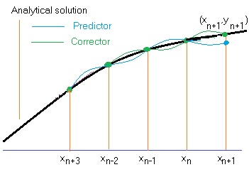
The Adams-Moulton methods is another predictor-corrector method. However, instead of sampling the slope in the interval [xn, xn+1] it uses slopes calculated at previous points. First a predictor uses a 4th order polynomial using the points (xn-3, yn-3), (xn-2, yn-2), (xn-1, yn-1), and (xn yn). and uses a weighted average of the slopes at those points to predict the y value at xn+1. It then uses a 4th order corrector polynomial using the points (xn-2, yn-2), (xn-1, yn-1), and (xn, yn) together with the predicted value at xn+1 and uses a weighted average of the slopes at these points to calculate a corrected y value at xn+1. (Sometimes, the correction is repeated to obtain an even better value but this program only corrects once.)
There is a problem with method. The values of three back points are required to calculate the first y value with this method. The initial starting point only provides 1 of those values. Some other method is required to get two more values. This program takes two steps with the Runge-Kutta method to obtain those points.
This method's error at each step is h5 so the error over and interval is proportional to h4 just as in the Runge-Kutta method although careful analysis shows it is about twice as large. Even so, it is often used because the Runge-Kutta method requires 4 evaluations of the y' function for each step while the Adams-Moulton method only requires 2 evaluations of the function in a carefully written program.
The boxes on this line are used for output - not input. The first box gives the final x value. (Normally this would be the ending x. However, if the step size doesn't divide evenly into the interval length, it may be slightly different. Numerical round off error may also cause it to be slightly different. Remember that even 0.1 can only be approximated on a binary computer.)
The next three box give the final values of y0, y1, and y2 at the indicated x value if those solutions were requested in the function boxes. In the boundary value mode the first two boxes give the final values of y and y'.
In boundary value problems, these are used to change the value of y' or y at the beginning x value. Use "Update y' " if the beginning value of y is fixed. If the beginning value of y' is fixed, use the "Update y" button.
Use these buttons only after firing at least one "practice" shot. If only one practice shot has been fired, it adjusts the indicated value a little. After two or more practice shots, it uses linear interpolation on the ending values to adjust the specified value. In a large class of problems, the third shot (after two practice shots and updates) will yield the correct boundary value at the ending x value. In other problems, it will be necessary to repeat the process over and over again. One can use the y or y' value in the above line to determine if the correct ending boundary value has been achieved.
The use of these buttons is not mandatory. One can update the appropriate value manually if desired. This may be especially useful after the first practice shot where the automated update may not be appropriate.
Clearing shot memory: As implied above, the apt keeps track the results of shots in order to determine if it is the first shot or if at least two shots have been fired. The shot count will be reset if certain changes are made (e.g. in the boundary conditions). The number of shots in memory is given in the "Ending y values" line. If necessary or if you just want to start over, you will want to clear the memory of previous shots. This is automatic if you change a function. If you are using one the examples and want to reset the shot count, you can pick a different example to clear the shot memory and then go back pick the desired example and make the desired changes.
Minimum x and Maximum x
are the left and right end points of the x axis. If the input boxes
are blank, the default values are the Beginning X and Ending X values.
If for some reason, you want a different range for x, the values of
can be specified as desired.
Minimum y and Maximum y,
if specified, are the end points of the y axis. If these fields are blank,
appropriate values will be calculated automatically based on the y values
of the function. They could be specified differently if desired.
If "Equal spacing" is true (checked) then the mins and maxs for x and y will be adjusted as needed in order to make the equal spacing possible.
Note: After you finish typing a minimum or maximum, press "Enter". The minimum and maximum values can be formulas which are evaluated the same way functions and values are evaluated. Just don't use x, y, v, or w in the formulas.
Sometimes it is useful to zoom in to see the results more closely. The Zoom In button does this. The domain is reduced by one fifth and centered at the last x value. If both the y minimum and x maximum are specified the range is reduced in a similar manner. Otherwise the range is determined in the usual manner. If the new domain or range is not appropriate, you may specify the x minimum or maximum or the y minimum or y maximum to show the appropriate domain or range.
The user can set the center by double click at the desired point.
Zoom out increases the domain by a factor of 5.
When Equal Spacing is checked, the units on the x and y axis are the same so a 45o line would look like a 45o line and circles will look like circles.
This feature is rarely used in DiffiEq2 but is included because it is part of the Grapher app.
For the sake of efficiency, DiffiEq2 stops redrawing graphs when nothing is changed. Checking Allow motion says to keep drawing. This is useful, for example, if one uses frameCount. E.g. 5 * sin(x + frameCount/10) or if you use the "s" slider.
The standard canvas is medium sized to allow the user see the canvas and many of the controls at the same time without having to scroll. This is convenient while developing a graph. But a larger graph is drawn above the original canvas and controls when the "Show enlarged canvas" item is checked or the "Enlargement ratio" is changed. When using this option, one will normally have to scroll up to see the larger graph and scroll down to see the original canvas and the control items. The enlarged canvas shows a magnified image of the original canvas except text elements are the same size as in the original.
Notes:
Sometimes it may be useful to allow changeable values in functions, beginning or final values or want an exact solution to match initial or boundary values. You can supply values for a, b, c, d, and e which can be used in the functions and other input boxes. The default value of these values is 0 when the input box is blank. You can use formulas which are evaluated the same way functions are evaluated. Just don't use x, y, v, or w in the formulas. See below for the special s value. You can use the value of one of the variables in another. For example, the expressions for a and b might be s/10 and 2 * d. Because one can use formulas for variables a, ...,e, the numerical values for these variables (rounded to 3 decimal places) is shown below the values.
Three of the values may have special meanings.
Value a will be used as the number of steps if the "Step size" box is empty providing it its value is a positive integer. This technique is used in example 2.
Whenever the values of Beginning x and/or Ending x are changed, then their values are stored in the b and e. This may be useful, for example, in order to automatically adjust the beginning y values according to the beginning x value. These values can be used for other purposes until the beginning and ending x values are changed. This technique is used in the first example. The beginning x value is in b and the ending x value is stored in e. But changing the values of b or e will not change the beginning or ending x values. This technique is also used in the first two boundary value problems.
The slider moves from 0 to 100 and is always an integer. If you move the slider, its value is sent to the s value input box. One can type a value from 0 to 100 in the s value input box to adjust the slider to that value. Anything else typed into that s value box is ignored and will be replaced by the value of the slider.
If the value range of the slider is not appropriate you can do something like the following: set d = s/10 and then use d in a formula, e.g. d * sin(x).
Important note: When "Allow motion" is false (not checked) the value of s is set when the mouse releases the slider but the value of s does not track the slider while the slider is moving. However, if "Allow motion" is true (checked) (and at least one function has been defined) the value of s tracks the slider.
Some additional variables have been added in order to make it easy to use values of some other values. Most of these values provide the value of a text box. Unfortunately the variable names are much less than intuitive.
| Variable | Associated box |
|---|---|
| Initial values | |
| g | Beginning x |
| p | Beginning y values first box: y0 or y |
| q | Beginning y values second box: y1 or y' |
| r | Beginning y values third box: y2 or y" |
| Calculated - not the text box value
Available only after using a method |
|
| H | Step size actually used in calculation |
| Calculated value from text box
Available only after using a method |
|
| G | Result at x =
(may differ from ending x because if step size doesn't come out evenly) |
| P | Result at x =, first y box for y0 or y |
| Q | Result at x =, second y box for y1 or y' |
| R | Result at x =, third y box for y2 or y" |
| Calculated value from text box
Available only after using a method for a boundary value problem |
|
| M | Ending y values, first box for y0 or y |
| N | Ending y values, second box for y1 or y' |
Example 7 uses G and M to locate the target for the right boundary value. Note that initially G will be 0 until one of the methods is used.
This value determines the number of times functions for y3, y4, and y5 are evaluated. The initial value of 200 is almost always adequate as that means these functions are evaluated at about every other pixel in the x direction. The numerical solutions are drawn as straight lines between the calculated values and this value does not effect them.
This button is useful if you have a copy of DiffiEq2 on your computer. If you set up a graph that you want to use again in another session, you can click this button and dialog box will show the information needed for the current plot to add it to the setupExamples() function in the DiffiEq2.pjs. You can copy the information and paste it into the function. You will have to provide an unique example number and a name for the graph. Formulas are shown in the order of the example numbers.
If a "," is included in a "word" special option w in function boxes, it will be replaced by "^$". The substitution is required because "," are used to separate items in the data. However, this is not a problem because the "^$" is automatically replaced by "," when used in a example.
If you click this button, the current setup saved as a new example which is added to the list of examples. You will be required to supply a name for the new example. The temporary example will only be available for the rest of current session.
After finishing a graph, it can be saved as an image file. Click the button. Depending on your browser, you may be asked if you want to save the file. In any case, you will probably find it your normal download folder with name diffiEq2.jpg. If you save more than one time, the multiple copies will normally be numbered. Your browser may have a button to give direct access to this folder. This option may work even if you are running DiffiEq2 on line.
The purpose of Show data option is to list the data values calculated by one of numerical methods. There are three options:
In any case, the output begins by showing the method and step size. It then lists any functions specified in the function input boxes. Initial values are shown for derivative functions. If one of the methods has been used, this is followed by column headings. "*" is used to denote columns for actual data not calculated by a method. Then the calculated values are shown line by line. "Actual" values are included if y3, y4, and/or y5 have been provided.
When the user types invalid info into one of the input boxes, a message is displayed on the top of the plot area. After fixing error, normally the error message will be hidden. Occasionally it may be necessary to click anywhere in the plot area to hide the message.
James Brink, 5/6/2021